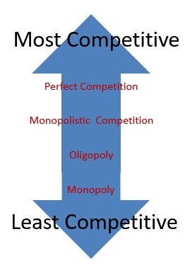
Keys to Understanding Perfectly Competitive Markets
Keys to Understanding Perfectly Competitive Markets
Updated 9/24/2020 Jacob Reed Like All Profit Maximizing Firms:
Produce the quantity where MR=MC
Price at Demand
Temporarily shut down when price falls below Average Variable Cost (AVC) at the profit maximizing quantity.
Profit/loss is determined by the gap between the ATC and the firm’s demand curve at the profit maximizing quantity (MR=MC).
Number of Sellers: Many
Product Difference: None. All products in this market are identical.
Ability to Affect price: None
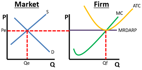
Graph: Usually drawn with 2 graphs. One for the market (AKA industry) and one for the firm. The market graph is a standard supply and demand graph with an equilibrium price and quantity. Since the firm is a price taker (no ability to affect price), the firm’s demand curve is horizontal (perfectly elastic) at the market price. This demand curve is also the firm’s average revenue (AR), marginal revenue (MR), and price (P). Together the 4 curves in one form what is often labeled MRDARP. The firm produces the quantity where MR=MC.
Note: The cost curves for perfect competition are the same as a monopoly and monopolistically competitive firm. The AVC and AFC are rarely needed in this graph.
Perfectly Competitive Market and Firm - Long Run Equilibrium
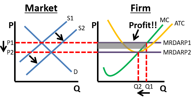
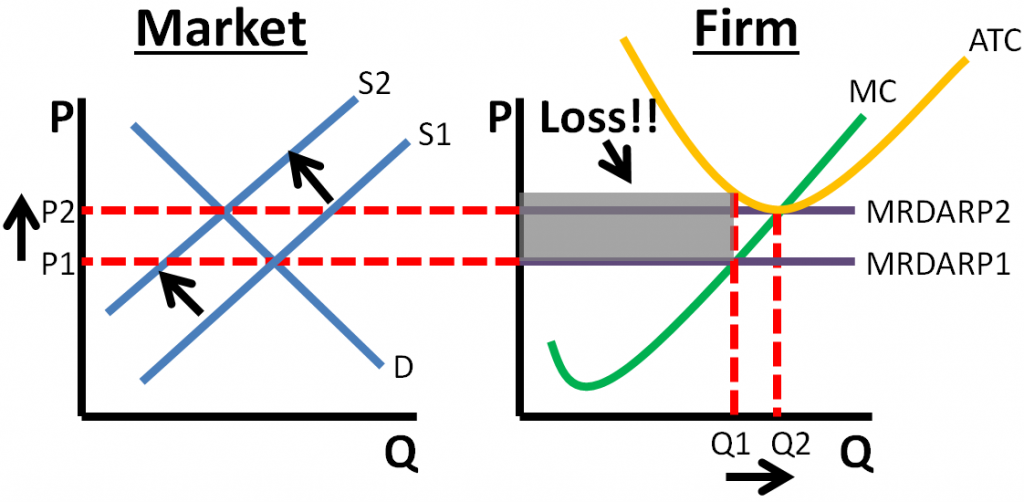
Barriers to entry: A barrier to entry is anything that makes it difficult for entrepreneurs to enter the market and compete. Barriers to entry can be high start up costs, customer loyalty, government regulation, etc. In perfectly competitive markets, barriers to entry are low. That means, when firms are earning economic profits, competing firms seek that profit and enter the market in the long run. When firms enter the market, prices fall and economic profit goes to zero. When firms are earning economic losses, firms exit the market (as resources will be more profitable elsewhere) in the long run, causing prices to rise until economic losses are zero. In the end, low barriers to entry (and exit) mean competitive markets earn zero economic profit in the long run.
On the graph, when firms enter the market it shifts the market supply curve to the right, decreasing the market price and MR=D=AR=P until firms break even. When there are economic losses in the short run, firms exit the market in the long run which shifts the market supply curve to the left, increasing price and MR=D=AR=P until the firm breaks even.
Note: Firms cannot enter or exit the market in the short run. The number of firms can only change in the long run.
Perfectly Competitive Market and Firm Short-Run Profit to Long-Run
Perfectly Competitive Market and Firm Short-Run Loss to Long-Run
Long-run Profit: No, due to the low barriers to entry.
Allocatively Efficient: Yes, because price equals marginal cost in both the short-run and long-run.
Productively Efficient: Productive efficiency occurs when the firm is producing at the minimum of the average total cost (ATC) curve (where it intersects the MC). In the short run, perfectly competitive firms are not productively efficient, but in the long run they are.
Firm’s supply curve: Below the ATC there is an average variable cost curve (AVC) that isn’t always drawn in . The minimum point on the AVC correlates to the lowest price a firm would be willing to accept. If the market price is above the AVC, the firm will produce the quantity where MR=MC. As the price falls, profit will fall but the firm will continue to produce where MR=MC. If the price continues to fall, the firm will produce lower quantities as long as the price stays above the AVC.
Firm Supply Curve (For Any Firm)
If the price falls below the AVC, the firm shuts down (temporarily) as the firm will only lose it’s fixed costs if it shuts down. Producing at a price below the AVC would cause the firm to lose more than their fixed costs. If the price equals the minimum of the AVC, the firm will produce that quantity; it is the lowest quantity the firm would produce. As a result, the firm’s supply curve is the MC curve above the AVC.
Note: This is true for all firms. The supply curve for all firms is the MC above the AVC.
Perfect competition total revenue and total cost: Profit maximizing firms produce where MR=MC. An alternative way to find the profit maximizing quantity is to look at a firm’s total cost and total revenue. A perfectly competitive firm’s total revenue curve rises at a constant rate (it is an upward sloping straight line). That is because the marginal revenue is equal to the price and does not change. When you graph total cost and total revenue on the same graph, you can also find the profit maximizing quantity by finding the quantity where the total revenue is farthest above the total cost. In the graph above, Qf would be the profit maximizing quantity. Q1 and Q2 both result in an economic loss.
Total Cost vs Total Revenue for Profit
Market long-run supply curve: The market supply curve is actually a short-run supply curve. That is because in the short run, the market can produce more at high prices and less at low prices. The long-run supply curve is a perfectly elastic (horizontal) curve at the bottom of the firm’s ATC. That is because the market price will always return to the bottom of the ATC in the long run. If there is an increase in demand, the price will increase and create short-term profits. Those profits will cause firms to enter the market increasing the market quantity even more, but decreasing the price back to the long-run price. If there is a decrease in demand, the price will fall and create short-term losses. Those losses will cause firms to exit the market decreasing the quantity more and returning the market price back to the bottom of the ATC. As a result, in the long-run the market can produce any quantity at the long-run price.
Long Run Market Supply Curve - Perfect Competition
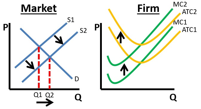
Increasing Cost Industry: Generally questions regarding perfectly competitive firms will be about constant cost industries. Those are industries where the firm’s cost curves do not shift based on the equilibrium output in the market.
You could see a question or two (on the AP Micro Exam) about an increasing cost industry. That would be a product where an increase in the market equilibrium quantity would cause an increase in costs for the individual firm. So an increase in Qe would cause the ATC and MC to shift upward for the firm.
Perfect Competition - Increasing Cost Industry
Increasing cost industries occur because the long run average total cost curve for the industry as a whole is upward sloping. Precious metals are an example increasing cost industry because as more gold and silver is produced (through mining) the cost of producing more constantly increases; as gold and silver become more and more difficult and costly to mine.
A decreasing cost industry is just the opposite. Cost curves will shift downward as industry output increases. This is as a result of the industry’s long-run average total cost curve sloping downward. These industries capture economies of scale. Microchips are an example of a product in a decreasing cost industry. The more that are produced, the cheaper production typically gets.